
The Specialist Is Now You
What AI enabled yesterday was a benchmark number. What AI enabled today is the individual, working alone, owning the whole pipeline from raw sequence to mechanistic call.

I reproduced Goodfire’s mechanistic variant-effect pipeline on cancer genes over a weekend. One box. Open weights. The payoff shows up whether or not the clinic is ready for it.

A BRCA1 variant lands in front of a clinician. The lab report says “variant of uncertain significance.” The oncologist looks at it, the genetic counselor looks at it, nobody can act. About thirty percent of oncogene variants in ClinVar (the public catalog of human genetic variants and their clinical labels) carry that same shrug. Patient leaves the appointment with no actionable call, no mechanism, no next step.
BRCA1 is a tumor suppressor. When it breaks, inherited breast and ovarian cancer risk goes up. A pathogenic variant calls for surveillance, sometimes surgery. A benign variant calls for a reassuring conversation. A VUS (variant of uncertain significance) calls for neither. The default is to wait until more families with the same variant get sequenced and the label firms up. Decades, in some cases.
This is the gap AlphaMissense partially fills. Google DeepMind trained it on missense variation (single-letter mutations that change the protein), and on that slice it is near the ceiling of what current data allows. But AlphaMissense is silent on everything that isn’t missense. Noncoding variants. Splice regions. Untranslated regions. Promoters. Synonymous changes (letter swaps that don’t change the protein but break splicing anyway). Insertions and deletions. Most of the interesting VUS space.
In March 2026, Goodfire shipped EVEE, a pipeline that scores every ClinVar variant, 4.2 million of them, and doesn’t just produce a pathogenicity score. It produces a disruption profile. Splice site broken. Regulatory element disrupted. Protein domain fold affected. Actionable explanations.
The catch was infrastructure. EVEE ran on Evo 2 40B (Arc Institute’s 40-billion-parameter DNA foundation model) on top-end data-center GPUs, with proprietary interpretability tooling and a team. A senior clinical geneticist at an academic cancer center couldn’t have reproduced that paper over a weekend. They’d need months of procurement and a six-figure budget, minimum.
I wanted to see what the approach looks like when you strip the proprietary layer out and run it on the kind of box a motivated lab could afford.
A year ago, mechanistic variant interpretation meant buying into somebody else’s stack. This year it is a workstation problem.
What Changed This Year
Three things quietly flipped, and together they make the story different.
Open foundation-scale DNA models. Evo 2 7B (the 7-billion-parameter sibling of the one Goodfire used) is on HuggingFace. Weights there, paper there, training recipe described. The smaller model is strong enough on variant effect out of the box, with no fine-tuning, to hold its own against specialized tools.
Open interpretability artifacts. Goodfire released a sparse autoencoder trained on Evo 2’s layer 26 (a specific layer deep inside the network), 32,768 features, public on HuggingFace. That’s the thing that turns a dense model activation into a sparse dictionary of “concepts the model learned about DNA.” Without it you’re guessing which channels matter. With it, you’re reading the model’s own internal vocabulary.
Consumer-adjacent GPU memory. The NVIDIA GB10 has 128 GB of unified memory. That’s enough to hold Evo 2 7B alongside 4,471 variant windows and a sparse autoencoder. The shift isn’t that data-center chips exist. It’s that “enough memory to do meaningful genomics interpretability” is no longer a facility-level decision.
Three years ago, any one of those three would have been the story. Today they compose. That’s the point.
What I Built
Six cancer genes. Two hereditary tumor suppressors (BRCA1, BRCA2). One pan-cancer tumor suppressor (TP53, the most-mutated gene in human cancer). Three oncogenes (KRAS, PIK3CA, EGFR) covering colorectal, lung, and breast signaling. Each picked because ClinVar has dense coverage and the clinical context is well-characterized.
For each variant I pulled an 8 kilobase (8,000-letter) genomic window centered on the position. That’s the reference version. Then I swapped in the mutant letter to get the patient-DNA version. Two runs through Evo 2 7B per variant, tap the activations at layer 26, save to disk. Five hundred and fifty-nine gigabytes of model activations, cached.
Then I compressed those activations. At every one of the 8,192 letter positions in each window, the model produced a 4,096-number vector describing what it “saw.” I reduced that to a per-variant summary by taking mean and standard deviation across positions. Two numbers per feature, 8,192 features total. Not covariance, nothing fancy. Call it diag pooling.
Feed that into a plain logistic regression (the simplest classifier there is, first-year-stats material). Five-fold cross-validation: train on four-fifths of the data, test on the last fifth, repeat five times, average. That’s the whole probe.
The probe is plain old logistic regression. That is not the part that’s new. What’s new is the thing feeding it.
The baselines were chosen to tell me what each layer was contributing. A k-mer floor (count short DNA strings in ref and alt, see if that alone separates pathogenic from benign) to confirm raw lexical signal can’t do this task. HyenaDNA, a different DNA foundation model, to test whether any such model would work or whether Evo 2 specifically matters. AlphaMissense precomputed scores, to benchmark against the specialist clinicians actually use.
End to end, including data prep, took a weekend of wall-clock and about 8 GPU-hours of compute on one box in a closet.
The Numbers
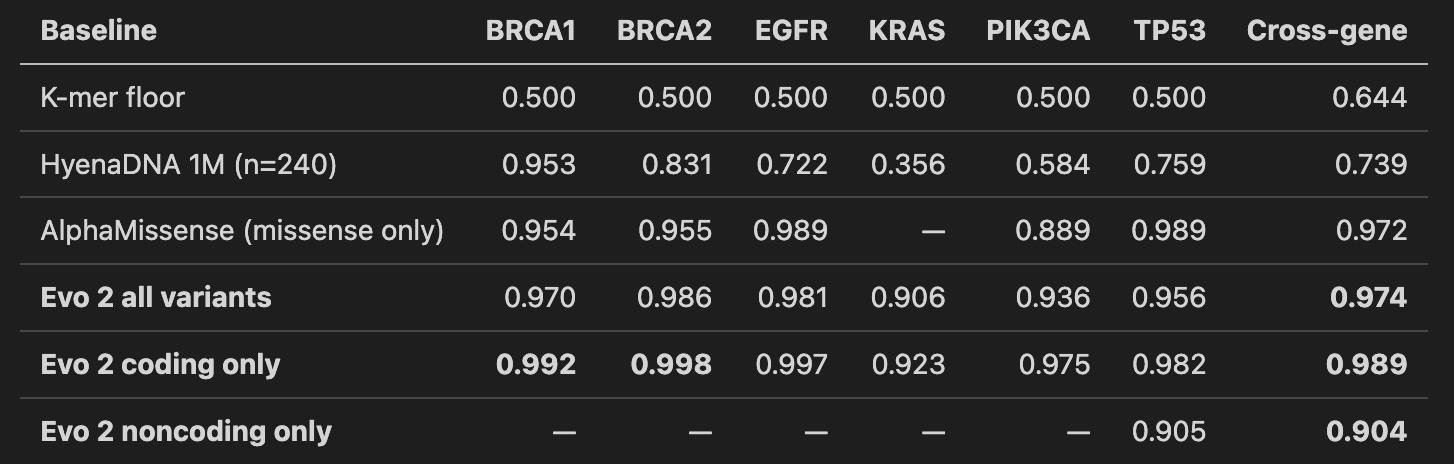
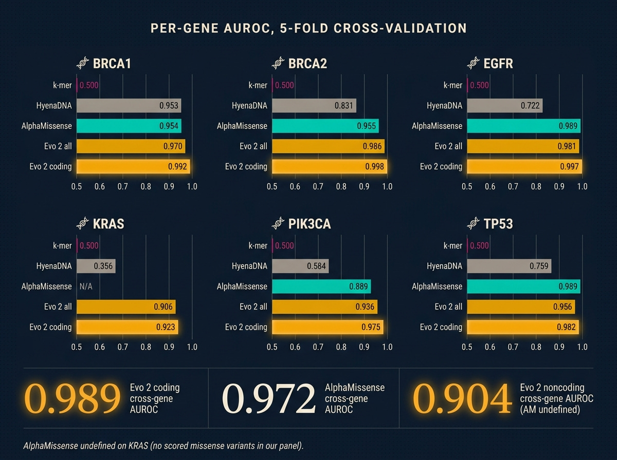
All numbers are AUROC (a 0.5-to-1.0 score where 0.5 is a coin flip and above 0.9 is strong medical-classifier territory), averaged across five cross-validation folds.
Three things to see.
Evo 2 beats the specialist on coding. Cross-gene 0.989 against AlphaMissense’s 0.972. Gene by gene, Evo 2 wins everywhere it plays. BRCA1 coding at 0.992 is stronger than the 0.94 Evo 2’s own paper reports on full-ClinVar training. I read that not as my reimplementation being better than Arc Institute’s, but as a focused oncogene panel being an easier subset of the full variant distribution. The panel matters.
K-mers cannot do this task. Every per-gene AUROC is exactly 0.5. Not noise. At 8 kb windows, a single-letter variant changes so little of the surrounding-letter-string statistics that a simple counter has nothing to grip. If your intuition says “can’t you just count the sequence differences,” this is the number that disproves it.
Noncoding is where the real coverage win lives. AlphaMissense is undefined on noncoding. Evo 2 gets 0.904. That is a modest-but-real 1,072-variant result with heavy class imbalance (most labeled noncoding are benign, only around 170 pathogenic across the panel). TP53 has enough labeled noncoding pathogenic for a per-gene fit and lands at 0.905. The other five genes ride the cross-gene probe. The result holds: these are variants AlphaMissense produces no score for, that Evo 2 produces a usable one for.
The Mechanistic Payoff
AlphaMissense gives a number. A sparse autoencoder on the right layer gives a reason.
This is the part a clinician can act on, and it’s the part that justifies doing the work at all.
I ran the public Goodfire sparse autoencoder (SAE) over Evo 2’s layer-26 activations for every variant. For each of the SAE’s 32,768 learned concepts, I measured how much the concept’s activity shifted between the reference window and the mutant window, then scored concepts by how much that shift separates pathogenic from benign variants within each gene. Rank descending.
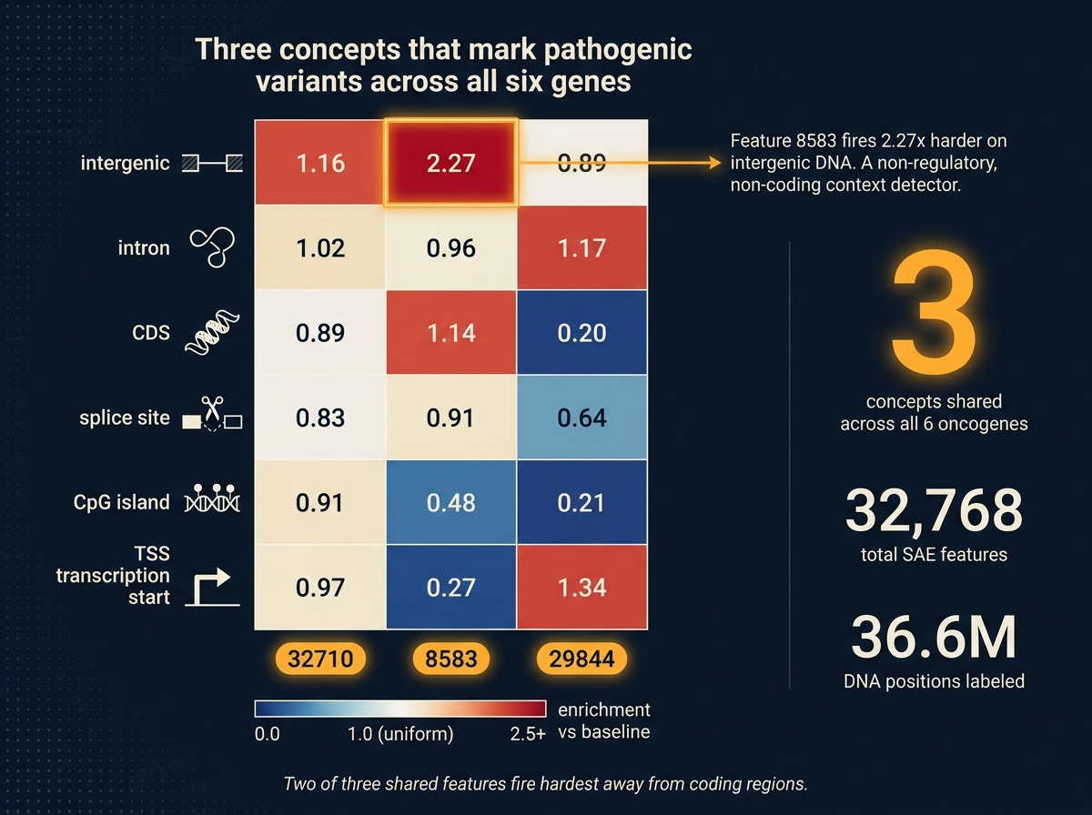
Three concepts (features 32710, 8583, 29844) land in the top-10 for every one of the six genes. Not different features for different genes, the same three across all six. That’s a candidate set of general disruption detectors: SAE concepts that light up whenever a pathogenic variant perturbs its context in a consistent direction, regardless of which oncogene is involved.
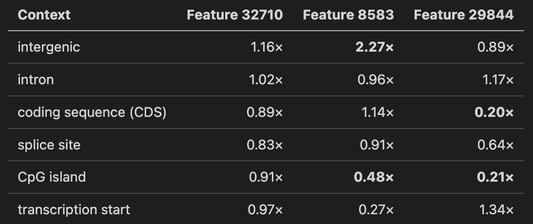
To ask what those three features are, I did a second pass. For every one of 36.6 million DNA positions across all variant reference windows, I labeled the position by its genomic context (using standard annotation databases): intergenic (between genes), intron (non-coding parts of genes), coding sequence, splice site (the signal that tells the cell where to join coding exons), CpG island (a gene-regulatory cluster), or transcription start (where a gene begins). Then I asked: where does each of the three shared features fire hardest?
The numbers below are enrichment over per-feature baseline. A value of 1.0 means “as expected.” A value of 2.0 means “fires twice as hard as average.”
Three readings.
Feature 32710 is a dispersed detector. Near-uniform across all contexts, high baseline activation. Probably a global sequence-complexity feature that modulates pathogenicity signal without being context-selective.
Feature 8583 is an intergenic-context detector. Fires 2.27 times harder on intergenic positions than average, less than half as hard on CpG islands and transcription start sites. A “non-regulatory, non-coding context” signature. When it responds to a pathogenic variant, the model is reacting to disruption of how the sequence looks away from canonical regulatory anchors.
Feature 29844 is coding-depleted. Five times less active in coding sequence than baseline, four times less on CpG islands. Enriched on transcription start sites and introns. Another “not canonical coding” detector, with a different signature from 8583.
Two of three shared pathogenicity features fire hardest in sequence contexts away from the coding region. That is a biological hypothesis the probe alone could not have produced. It says: Evo 2’s internal notion of “this variant is pathogenic” derives substantially from the model’s expectation of what should be at that position, and that expectation is shaped by whether the region looks coding-like or not. Break that expectation, the pathogenicity signal spikes.
Whether those three features map to known biology or to something Evo 2 learned that nobody has named yet is the next question. Having them identified, ranked, and characterized to this level is already more than a probe on its own could have produced.
What Didn’t Work
Two threads I’d have liked to report as wins.
Covariance pooling. EVEE’s original paper uses covariance pooling, a more sophisticated way of summarizing the model’s per-position activations (it tracks how features vary together, not just individually). I reimplemented it faithfully, ran it, and it lost to plain diag pooling on every single gene. Cross-gene covariance 0.920 against diag 0.974. On KRAS and PIK3CA the gap was 0.08 to 0.13 AUROC. Why? The fancier summary produces roughly 16,000 features per variant, and at roughly 1,000 variants per gene, the probe has too many knobs and not enough data to constrain them. EVEE trained on 4.2 million variants. At that scale, the parameter count gets earned. On a six-gene panel, it doesn’t.
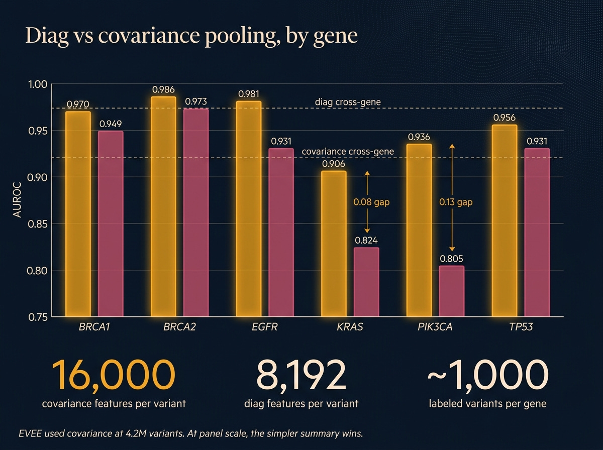
The lesson isn’t that covariance is wrong. It’s that faithful reimplementation of a method built for a different data regime can lose to the simpler approach. Diag is good enough at panel scale, and probably for any lab-scale project that isn’t doing a full-ClinVar retrain.
Regulatory and structural auxiliary probes. I trained probes to predict whether each variant overlaps a known regulatory switch (from the ENCODE database; AUROC 0.706) and whether it sits inside a known protein functional domain (from UniProt; 0.823 on the yes/no version, 0.693 on the which-domain version). The regulatory probe came in below the 0.80 bar I’d set. The structural binary cleared it; the multi-class domain-identity probe did not.
The useful result in the pile is the structural binary: Evo 2 can tell, from sequence alone, whether a variant sits inside an annotated protein domain. A capability, not a headline. Noted for the next pass.
Who Can Do This Now
A clinical geneticist with a 128-GB GPU workstation (the new consumer-grade GB10, or a rented data-center H100) can produce per-variant disruption profiles for a focused gene panel over a weekend. Not a full-ClinVar retrain. A targeted, interpretable pipeline on the panel they care about.
That’s the shift. The infrastructure moat collapsed. What used to require a proprietary stack and a research team is now something an individual can own end to end, from data pull to mechanistic output, with only open weights and open interpretability tools.
This doesn’t mean every clinical VUS gets an explanation tomorrow. It means the work to get there is accessible to the people who actually see the variants and talk to the patients. That changes who gets to contribute.
One More Year
A year ago, the honest answer to “can a clinical geneticist run their own variant interpretation pipeline?” was no. You needed a team, a stack, a budget most labs couldn’t justify.
Today I did it on one box, over a weekend, with open weights and open interpretability artifacts. Not as well as Goodfire did at 4.2 million variants. Well enough to beat the specialist tool most clinicians actually use on coding variants, extend it into noncoding where that tool is silent, and produce mechanistic feature-level explanations that point at real biology.
The model is downloadable. The interpretability artifact is downloadable. The code runs on hardware you can buy. None of this needed a cluster.
What AI enabled yesterday was a benchmark number. What AI enabled today is the individual, working alone, owning the whole pipeline from raw sequence to mechanistic call.
The specialist is now you.